Third-year electronics, electrical engineering and control student at Sorbonne University, with a mathematics minor. I design circuits and robotic prototypes, from sensors to embedded software. I also share my photography and 3D work.
Electronics, robotics and software: my projects, design choices and current progress.
Photography
3D modelling
About
I am Benjamin Piras, a third-year student at Sorbonne University, majoring in electronics, electrical engineering and control (EEA), with a mathematics minor. I am interested in the complete system: sensors, circuits, acquisition, programming and control.
StudiesThird-year EEA major, mathematics minor — Sorbonne University
During my internship at the Institute of Intelligent Systems and Robotics (ISIR), I worked on an instrumented robotic hand prototype. From component selection and PCB design to sensor processing, this experience brought electronics and robotics together in one project.
A tactile sensing system for a robotic hand needs an acquisition chain that can read distributed sensors, transmit their measurements and make the data usable. I designed this chain during my research internship at ISIR, Sorbonne University, supervised by Nizar Ouarti.
The architecture connects one main controller board to 15 phalanx boards, intended to accommodate 45 three-axis Hall-effect sensors. My work covered component selection, circuit schematics and PCB layout, embedded software, wireless communication and measurement interfaces. The prototype was experimentally validated with nine sensors across three phalanges.
The intended tactile principle uses small magnets embedded in a deformable surface. Contact changes their position relative to the sensors and therefore the measured magnetic field. The acquisition chain captures these variations; estimating contact force requires subsequent mechanical calibration.
Architecture
Communication
Validation
1 main board · 15 planned sensor boards 3 TMAG5273 sensors per phalanx
1 MHz I²C 2 Mbit/s UART · ESP-NOW V2
9 sensors across 3 phalanges Reception on the order of 100 frames/s
01 — One main board and fifteen sensor PCBs
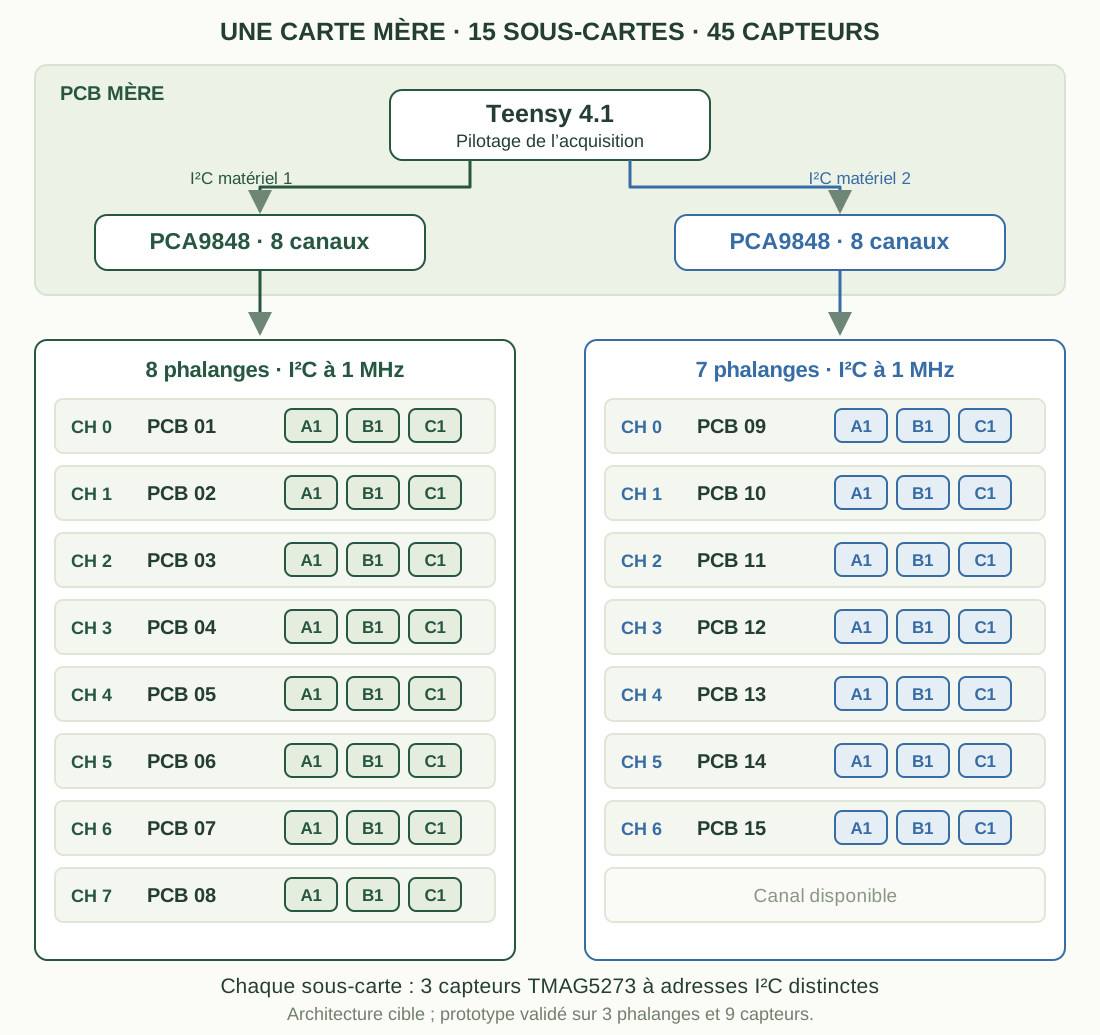
Each phalanx board contains three TMAG5273 sensors, labelled A1, B1 and C1. Their different I²C addresses allow them to share a local bus. The main board collects the measurements using a Teensy 4.1 and two eight-channel PCA9848 switches.
Each switch is connected to a separate hardware I²C controller on the Teensy. Its channels select the sensor boards: the firmware selects a phalanx, reads its three sensors, then proceeds to the next one. Identical sensor addresses can therefore be reused on separate branches while keeping the wiring manageable.
Target architecture for a complete hand: 15 sensor PCBs and 45 sensors. The 8 + 7 distribution illustrates how the two switches can be used, leaving one channel available. Hardware tests covered three phalanges.
The TMAG5273 was selected for its three-axis measurements, configurable range, internal averaging and I²C interface up to 1 MHz. A SPI solution was considered, but the selection lines required by the proposed direct topology would have complicated PCB and cable routing. Multiplexed I²C offered a suitable compromise for this distributed architecture.
02 — From circuit schematics to hardware
I separated the electronics into a main board for acquisition, communication and power management, and smaller phalanx PCBs for positioning the sensing points close to the surface being instrumented. This modular approach made it possible to test individual subsystems before mechanical integration.
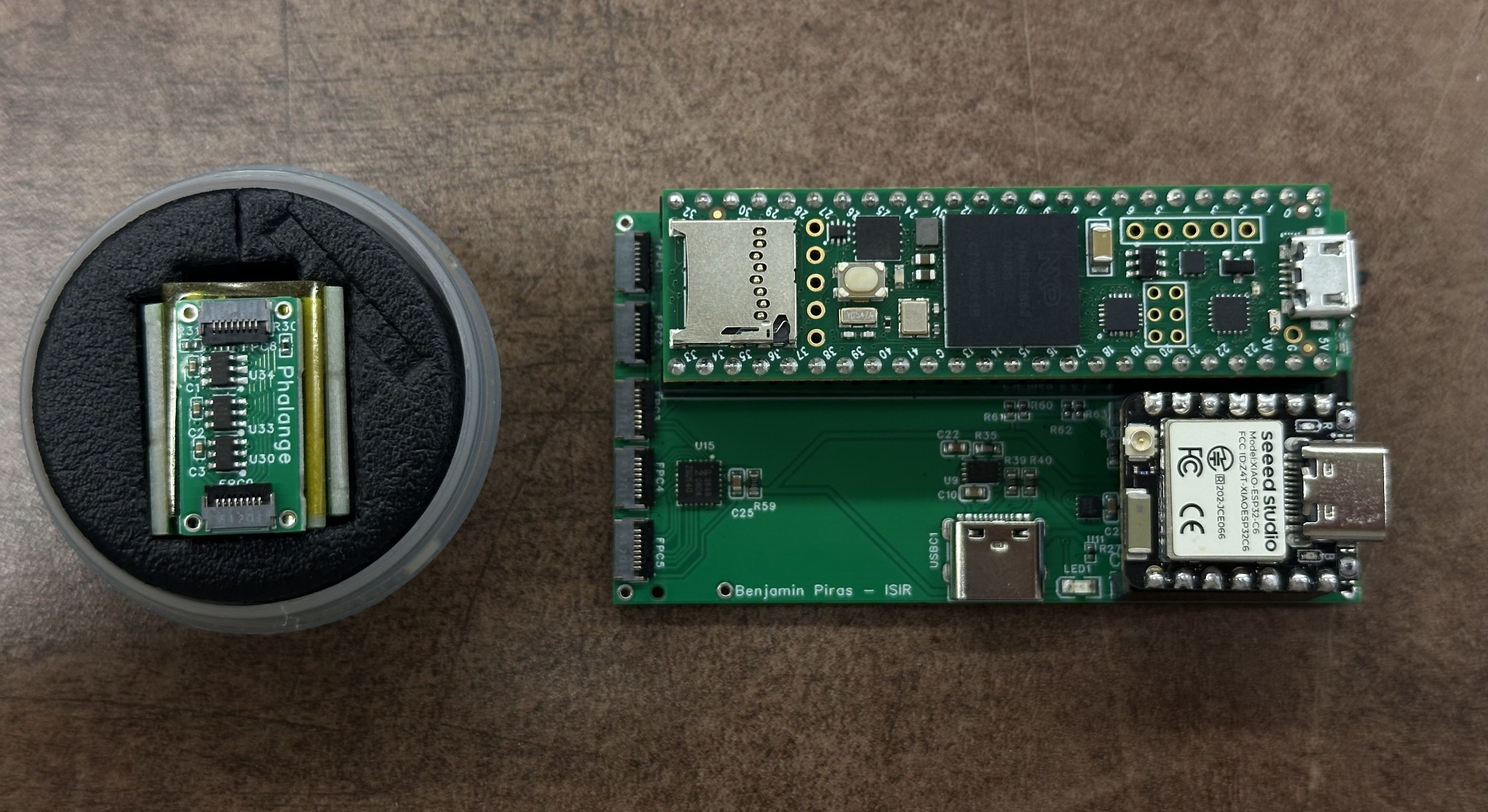
Hardware prototype: the main board on the right, with its Teensy 4.1 and ESP32-C6, and one three-sensor phalanx PCB on the left.
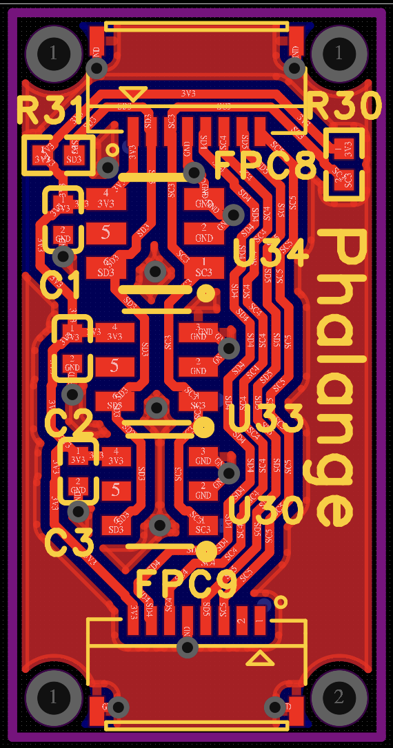
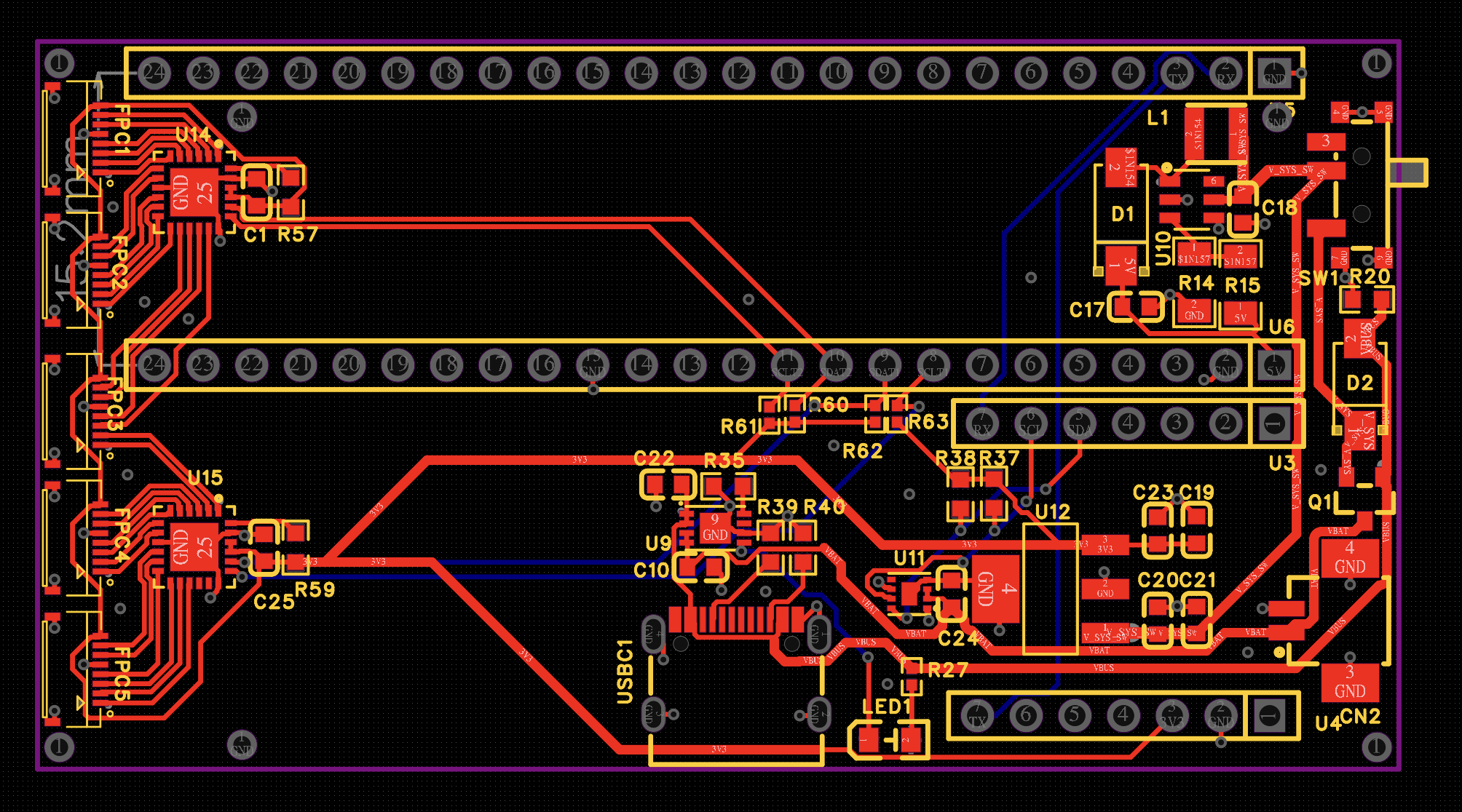
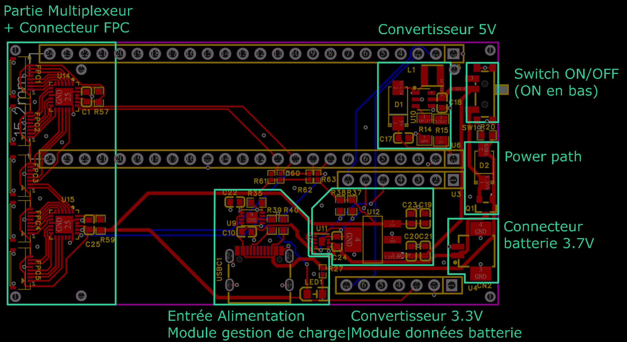
Phalanx PCB: three sensors and the connections routed to the FPC connectors.Main PCB: phalanx connections, microcontroller sockets, I²C multiplexing and power circuitry.
The layout evolved to improve connector orientation, simplify routing and adapt power-track widths to expected currents. The main board measures approximately 71 × 38 mm. The microcontroller modules are socketed so they can be replaced during hardware debugging.
View the main board’s functional blocksFunctional blocks of the main board: multiplexers and FPC connectors on the left, with power conversion, charging and battery connections below and on the right.
The system accepts USB-C power or a nominal 3.7 V, 1,200 mAh LiPo battery. A boost converter provides the 5 V rail and a regulator supplies 3.3 V. An MCP73831 manages charging, a power-path circuit gives priority to USB when connected, and a MAX17048 reports battery voltage and estimated state of charge.
Bring-up began with rail voltages, operation under load, temperature checks and firmware upload. Communications were first tested with simulated data, followed by real sensor readings. Battery tests revealed voltage dips that require further investigation, particularly during radio transmission.
03 — Transmitting measurements to the computer
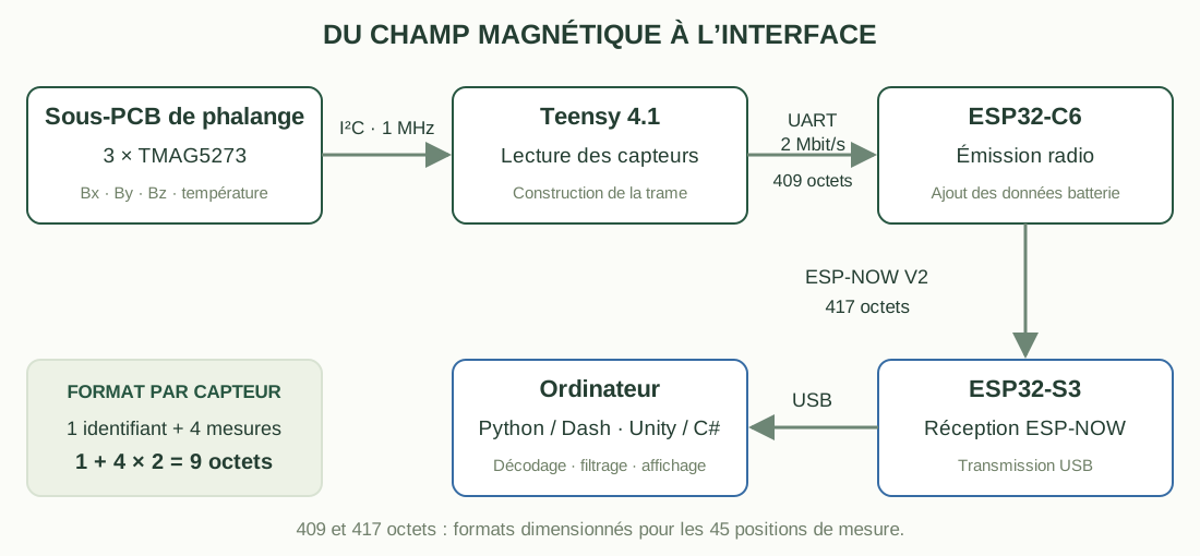
The Teensy reads the sensors over I²C and transfers a frame to the ESP32-C6 over a 2 Mbit/s UART. The ESP32-C6 appends battery information and sends the packet over ESP-NOW V2 to an ESP32-S3 receiver connected to the computer by USB.
Acquisition and communication chain. Frame sizes refer to the format designed for all 45 sensor positions.
Each sensor occupies nine bytes: one identifier and four two-byte values for Bx, By, Bz and internal temperature. The 45 positions account for 405 payload bytes. Delimiters bring the UART frame to 409 bytes, then battery information increases the ESP-NOW frame to 417 bytes.
The computer does not necessarily receive a complete frame in one read. I implemented buffered reconstruction that searches for start markers, waits for the expected length and verifies the end markers. The format is therefore independent of how the USB stream is split. An application-level CRC covering the entire frame remains a possible improvement.
TUART=2×106409×10≃2.05ms
This theoretical duration includes ten transmitted bits per byte in UART 8N1. It describes one transfer stage; end-to-end latency also includes acquisition, radio communication, processing and display.
04 — Processing data without blocking the display
The sensors operated in continuous-conversion mode, with a ±40 mT range and 8× hardware averaging. Raw values are converted into physical units before analysis. Transporting results as 16-bit words does not imply 16 bits of effective measurement resolution.
An exponential moving average stabilises the magnetic components:
Sn=αYn+(1−α)Sn−1
The coefficient controls the trade-off between smoothing and responsiveness. For α = 0.1 and a nominal 10 ms sampling period, the equivalent time constant is approximately 95 ms. This filtering delay is separate from communication time.
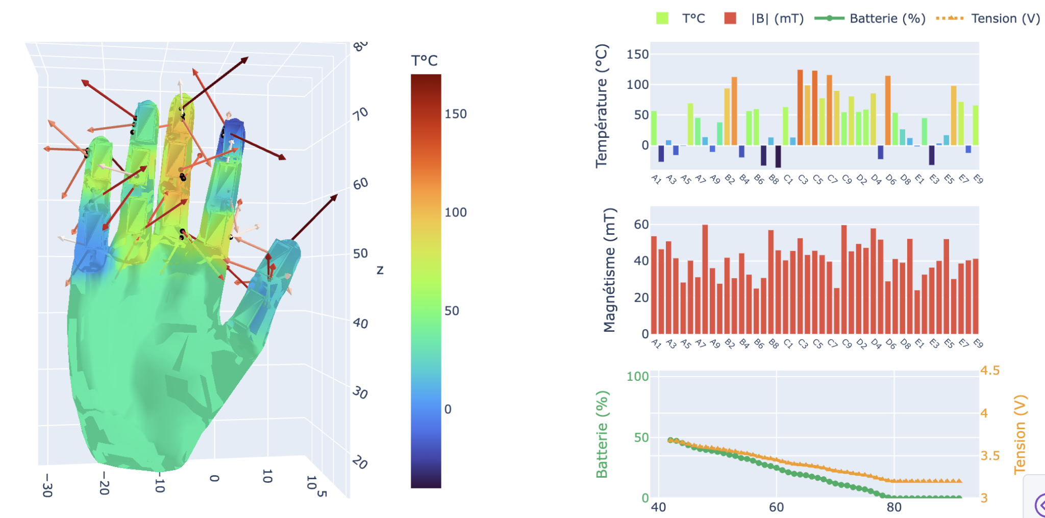
I developed Python interfaces with Dash and Plotly for observing signals and exporting CSV recordings. An initial 3D view supported interface development while the boards were being manufactured. A Unity/C# interface then separated background serial reception from graphical rendering. A lock protects copies of the shared arrays so measurements from different frames are not mixed.
Initial Dash/Plotly visualisation using simulated data. The temperatures and battery discharge shown here are not experimental results.
Video demonstrations
Dash/Plotly prototype: the hand visualisation and live chart updates using simulated data. · 35 s
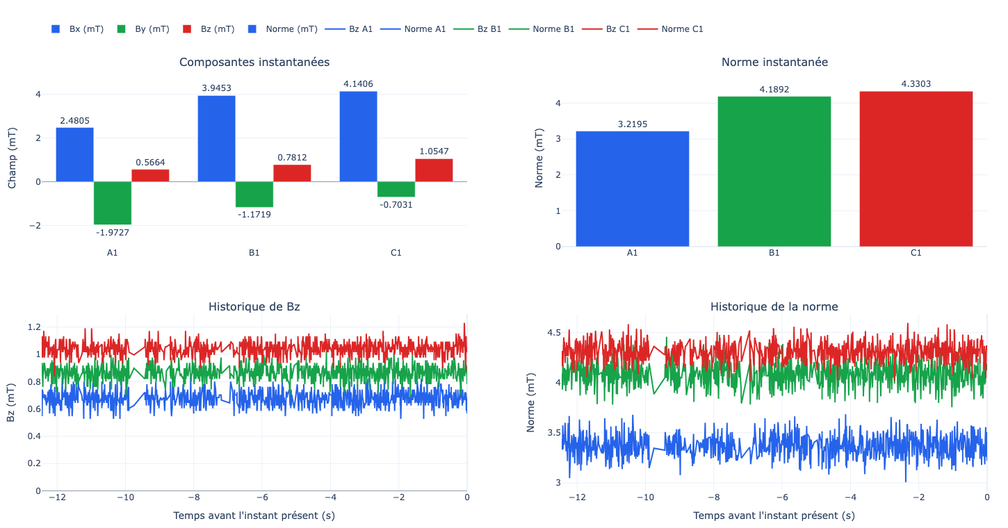
Dedicated phalanx measurement interface: instantaneous components and magnitudes, Bz history and field-magnitude history for the three sensors.
Observed reception was on the order of 100 frames per second. This is distinct from screen refresh rate and does not constitute an end-to-end latency measurement.
05 — Characterising background noise and distance response
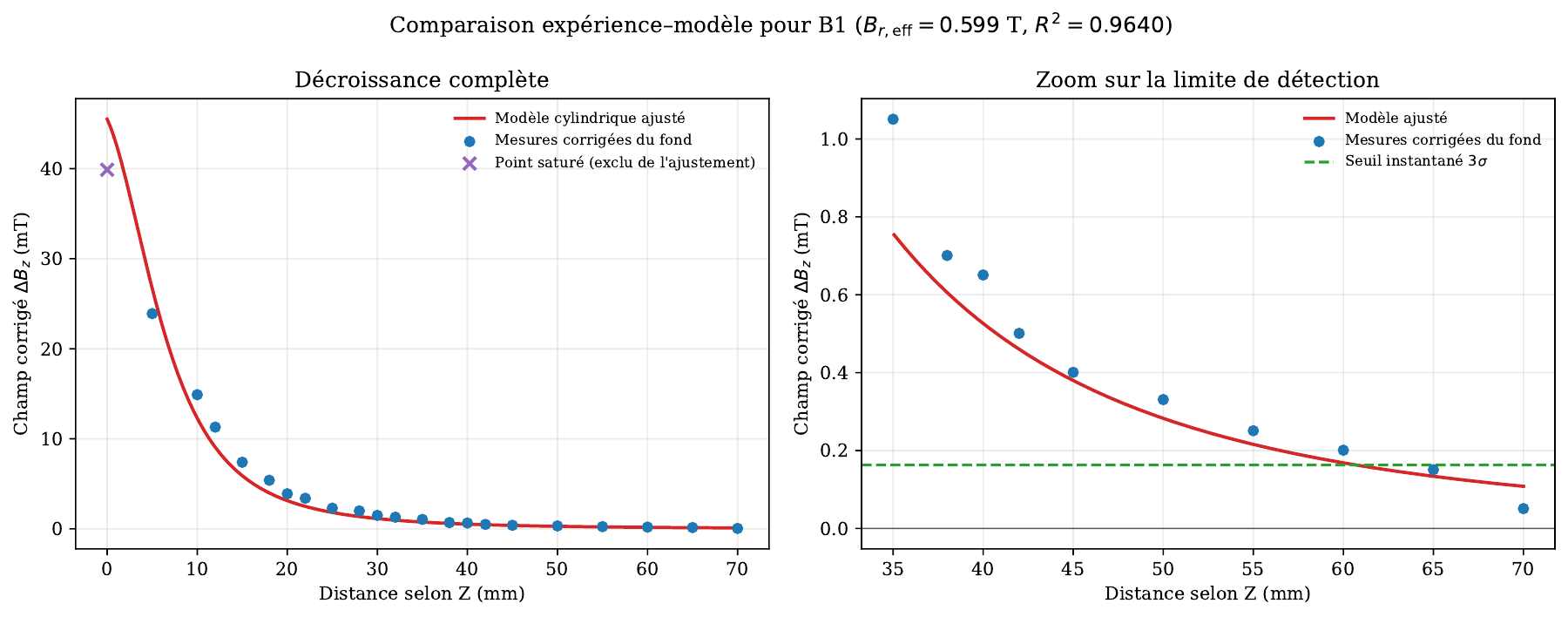
Magnetic characterisation mainly used one phalanx and a cylindrical neodymium magnet measuring 19 mm in diameter and 1.5 mm thick. Distance was set manually using a ruler, with an estimated positioning uncertainty of approximately 1 mm.
A background recording without an intentional magnetic source provided 5,966 samples per sensor. For B1, measured standard deviations were approximately 0.111 mT along X and 0.054 mT along Z. The chosen instantaneous three-standard-deviation thresholds were therefore 0.333 mT and 0.163 mT.
After background subtraction, Z-axis measurements were compared with a cylindrical-magnet model. The contact reading reached approximately 39.98 mT, near the configured saturation limit, and was excluded from the fit.
Bz decay compared with the cylindrical-magnet model, with R² ≈ 0.964. In this configuration, the instantaneous threshold is crossed between 60 and 65 mm.
Along X, the PCB edge added approximately 3.1 mm to the nominal distance, in addition to the sensitive point’s offset within the package. This geometry explains part of the difference between the curves. The instantaneous detection limit was between 40 and 50 mm in this configuration, compared with 60–65 mm along Z.
06 — Understanding coupling between adjacent sensors
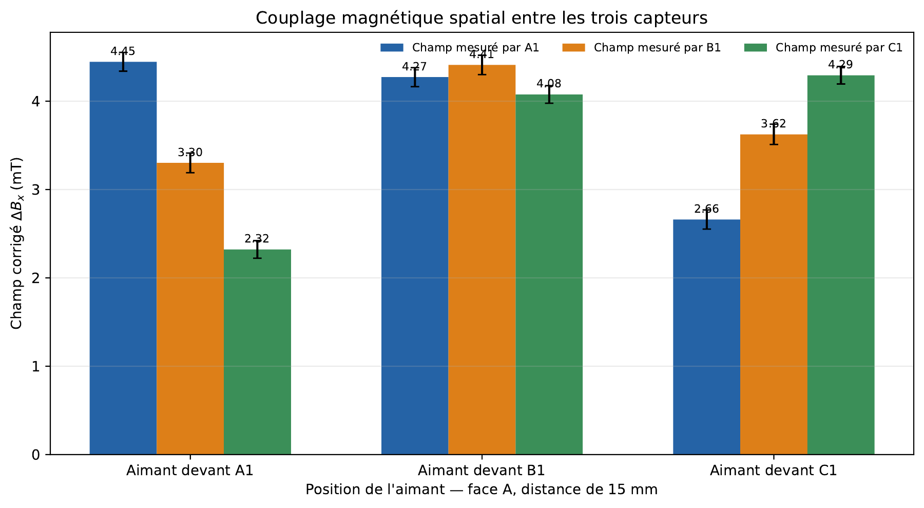
A source positioned in front of one sensor also affects its neighbours. With the magnet 15 mm in front of B1, A1 and C1 reached approximately 97% and 92% of B1’s response. The graph compares all three source positions.
Spatial coupling at 15 mm. Multiple sensors respond to the same source, so future contact localisation must consider the field distribution.
An independent threshold on each sensor is therefore insufficient to identify a contact location. Sensor spacing, magnet geometry and processing of all three components need to be studied together.
07 — Testing two magnetic sources
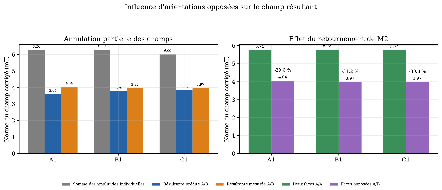
Two magnets were positioned in front of A1 and C1 at 15 mm. Background-corrected measurements of each source were used to predict their combined field through vector addition:
ΔBpredicted=ΔBM1+ΔBM2
The addition applies to Bx, By and Bz rather than directly to their magnitudes. Reversing one magnet partially cancelled some components, reducing the resulting magnitude by approximately 30% compared with the same-orientation configuration.
Effect of relative magnet orientation. Reversing M2 reduced the magnitude by 29.6%, 31.2% and 30.8% on A1, B1 and C1.
The expected trend was observed, with quantitative differences still sensitive to positioning. A low resultant field does not necessarily indicate the absence of magnetic sources: several contributions can partially cancel.
08 — Project outcome and further development
The project delivered a functional sensor-to-interface chain: designed and debugged boards, acquisition from nine sensors, wireless transmission, and visualisation and recording tools. It connects electronic design, embedded software and experimental analysis within one prototype.
Next steps include validating all 45 sensor positions, improving positioning repeatability and integrating the deformable surface carrying the magnets. Mechanical calibration will then be required to relate field changes to displacement and contact force. Battery behaviour and end-to-end latency also require additional measurements.
Towards a centralised ESP32-P4 architecture
A possible revision would consolidate acquisition and wired data transfer onto an ESP32-P4. Its two main I²C controllers could support a similar two-branch organisation, but they are documented up to 400 kHz, compared with 1 MHz in the current prototype. Acquisition timing, pin allocation, drivers and scheduling would therefore need to be reassessed.
A 10/100 Mbit/s Ethernet variant with an external PHY could send measurements directly to a computer or Raspberry Pi. Such a gateway could be administered over SSH; direct SSH access to the microcontroller would require a dedicated server in its firmware.
The P4 has no integrated Wi-Fi radio, so retaining ESP-NOW would require a wireless companion. Consolidation onto one microcontroller is therefore particularly relevant to a wired Ethernet or USB version, to be evaluated for size, power consumption and latency.